KL Divergence: Forward vs Reverse?
Discussions about the choices of forward / reverse KL divergence.
Kullback-Leibler Divergence, or KL Divergence is a measure on how “off” two probability distributions \(P(X)\) and \(Q(X)\) are. It measures the distance between two probability distributions.
Generally, KL divergence could be computed as follows:
\[\text{KL}(P(X)\parallel Q(X))=\sum_{x\in X}P(x)\cdot\log\frac{P(x)}{Q(x)}.\]That is, for all random variable $x\in X$, KL divergence computes the weighted on the difference between those distributions at $x$.
It is easy to observe that KL is NOT a symmetric metric to \(P(X)\) and \(Q(X)\), that is, in most cases \(\text{KL}(P(X)\parallel Q(X)) \neq \text{KL}(Q(X)\parallel P(X))\).
BTW, the symmetric version of KL is called Jenson-Shanon Divergence, formatted as
\[\text{JSD}(P\parallel Q)=\frac{1}{2}\cdot \text{KL}(P\parallel M) + \frac{1}{2}\cdot \text{KL}(Q\parallel M),\]where \(M=\frac{1}{2}\cdot(P+Q)\), is a mixture distribution of \(P\) and \(Q\).
So, here comes the question, if we assume \(P\) as the true distribution we want to approximate and \(Q\) is the approximate distribution, should we optimize towards \(\text{KL}(P\parallel Q)\) or \(\text{KL}(Q\parallel P)\)?
Generally, in such cases, we denote \(\text{KL}(P\parallel Q)\) and \(\text{KL}(Q\parallel P)\) as forward-KL and reverse-KL separately.
Forward-KL
In forward-KL, \(P\) acts as the weight factor. Consider \(P(x)=0\) for a specific \(x\), then the term \(P(x)\cdot\log\frac{P(x)}{Q(x)}\) would always be zero. Simply put, when \(P(x)=0\), it doesn’t matter that how different \(P\) and \(Q\) is at this point. As a result, we would ignore the affect of \(Q(x)\) here.
Hence, during the optimization, the different between \(P(x)\) and \(Q(x)\) will be minimized only when \(P(x) > 0\).
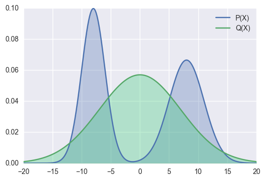
Let’s see some visual examples.

In the above example, the right hand side mode is not covered by \(Q\), but \(P(x) > 0\). Therefore, the KL divergence would be big.
In this example, \(Q\) covers more areas compared to the previous one. As a result, the KL divergence would be smaller.
Intuitively, forward-KL is also called zero-avoiding, as it avoids \(Q(x)=0\) whenever \(P(x)>0\).
Reverse-KL
As we switch the positions of the two distribution in the formula, we get reverse-KL, with \(Q\) as the weight AND the approximate distribution.
When \(Q(x) = 0\), again we ignore the value of \(P(x)\) at these points. When \(Q(x)>0\), we should minimize their distances here to achieve a lower KL divergence. In such cases, the first example, which has a larger forward-KL divergence, would be the desirable outcome under the evaluation of reverse-KL. That is, for Reverse KL, it is better to fit just some portion of \(P\), as long as that approximate is good.
As those properties suggest, this form of KL Divergence is known as zero forcing, as it forces \(Q\) to be 0 on some areas, even if \(P(x) > 0\).
Conclusion
Back to the question, the answer would be “it always depends”. We should choose the proper KL suitable to our problems.
Especially, in Bayesian Inference, in VAE (Variational Auto Encoder), Reverse KL is widely used.